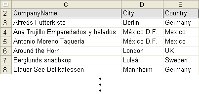
Consider a table containing fields such as Country and City:

Count customers by country

1. Open Insert → Pivot Table.
2. Select the customers table and click Source Range.
3. Select Country as the only Row field.
4. Select Count as the default function.
5. Choose a destination cell and click Insert.

Count customers by country and city

1. Open Insert → Pivot Table.
2. Select the customers table and click Source Range.
3. Select Country as the first Row field.
4. Select City as the second Row field.
5. Select Count as the default function.
6. Choose a destination cell and click Insert.

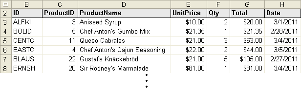
Consider a table containing fields such as ProductName, Date, Qty, and Total:

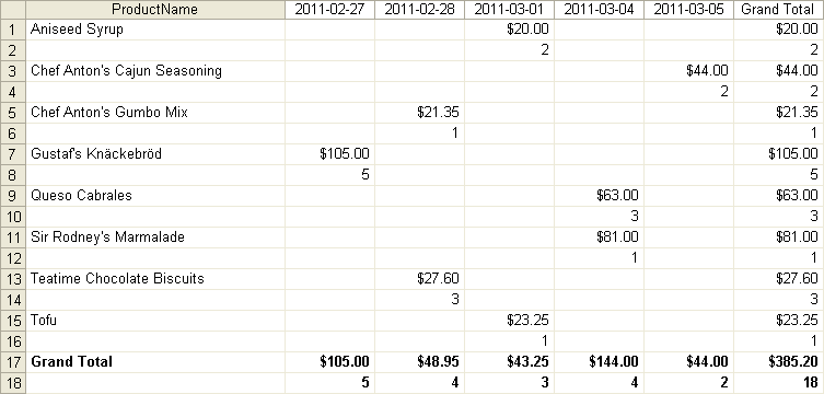
Sales volume by day

1. Open Insert → Pivot Table.
2. Select the products table and click Source Range.
3. Select ProductName as the only Row field.
4. Select Date as the only Column field.
5. Select Qty as the only Data field and choose Sum.
6. Choose a destination cell and click Insert.

Sales volume and quantity by day

1. Open Insert → Pivot Table.
2. Select the products table and click Source Range.
3. Select ProductName as the only Row field.
4. Select Date as the only Column field.
5. Select Total as the first Data field and choose Sum.
6. Select Qty as the second Data field and choose Sum.
7. Choose a destination cell and click Insert.

PIVOT formulas have the following form:

pivotData(source, rows, columns, data, functions, options [, field1, filter1, field2, filter2, ...])

This formula creates and returns a pivot table for the data in the source range.

3.1 Row, Column, and Data Fields

The rows, columns, and data parameters are arrays containing field indices. Indices are 1‑based and relative to the top‑left corner of the source range.

Examples:

{1, 5}, {4}, {1}

Incorrect indices cause #VALUE!. In GS-Calc 9.0, the columns array may contain only one element. If data fields are omitted, the last row field and the default pivot function are used.

3.2 Functions

The functions argument is an array of predefined constants:

• PIVOT::Sum — sum of values
• PIVOT::SumPositive — sum of positive values only
• PIVOT::SumNegative — sum of negative values only
• PIVOT::SumSquares — sum of squares
• PIVOT::Count — count of non‑empty values
• PIVOT::CountPositive — count of positive values
• PIVOT::CountNegative — count of negative values
• PIVOT::CountZeroes — count of zero values
• PIVOT::Mean
• PIVOT::Geomean
• PIVOT::Harmean
• PIVOT::Min — minimum value
• PIVOT::Max — maximum value
• PIVOT::Quartile1
• PIVOT::Median
• PIVOT::Quartile3
• PIVOT::Var
• PIVOT::VarP
• PIVOT::Stdev
• PIVOT::StdevP
• PIVOT::Skew
• PIVOT::Kurt
• PIVOT::Mode

Examples:

{PIVOT::Sum}

{PIVOT::Sum, PIVOT::Count}

3.3 Required Column Field or Grand Totals

You must specify either:

• PIVOT::ColumnGrandTotals
• or at least one column field

Otherwise the function returns #NUM!.

3.4 Options (FULL descriptions preserved)

The options parameter may be a sum of:

• PIVOT::ColumnGrandTotals (1) — display column grand totals in the last column
• PIVOT::RowGrandTotals (2) — include row grand totals in the last row
• PIVOT::SubTotals (4) — include subtotals (for pivot tables with 2+ row fields)
• PIVOT::ShowZeroes (8) — show zeroes for empty data fields; otherwise empty subtotals appear as #N/A!
• PIVOT::RepeatRowFields (16) — display all row field values, even duplicates
• PIVOT::CaseSensitive (218) — use case‑sensitive comparison when filtering
• PIVOT::SortRowsDescending (256) — sort output rows in descending order
• PIVOT::SortColumnsDescending (512) — sort output columns in descending order
• PIVOT::NoSourceFieldNames (1024) — source range contains no field names; use “Field n.” instead
• PIVOT::IgnorePunctuation (16384) — ignore certain punctuation marks when sorting/filtering
• PIVOT::NeutralSortOrder (32768) — use language‑neutral comparison
• PIVOT::Pattern (65536) — treat filters not starting with (=, >, >=, <, <=) as wildcard patterns
• PIVOT::HorzData (131072) — generate multiple data field values in single rows

Examples:

{PIVOT::ColumnGrandTotals}

{PIVOT::ColumnGrandTotals + PIVOT::RowGrandTotals + PIVOT::SubTotals}

3.5 Filters

Optional [field, filter] pairs specify filtering conditions. Only records matching all conditions are included.

Filters may be:

• A text string beginning with =, >, >=, <, <=
• A number
• A wildcard pattern using ? or * (escape with ~? or ~*)

3.6 Examples

=pivotData(C3:H19, {1},,, {PIVOT::Sum}, PIVOT::ColumnGrandTotals)

=pivotData(sheet1!C3:H19, {1}, {2}, {3, 4}, {PIVOT::Sum, PIVOT::Count}, PIVOT::RowGrandTotals + PIVOT::ColumnGrandTotals + PIVOT::SubTotals)

=pivotData(sheet1!B3:F8, {5, 1}, {3},, {PIVOT::Sum}, PIVOT::RowGrandTotals + PIVOT::ColumnGrandTotals + PIVOT::SubTotals, 2, "Jones", 4, ">2010-01-01")